In the context of my work with the computer vision platform VisionLit, I delve into the utilization of images for the identification of objects, reading QR/Barcodes, and the automatic extraction of information from documents such as identity cards. These functionalities are made available through our Application Programming Interfaces (APIs). It is pertinent, in further exploring our main topic, to delve into some fundamental principles of image processing. Understanding these principles is vital for the development of both efficient and reliable algorithms. Hence, this article aims to detail not only the inherent structure of a digital image but also to illuminate the most commonly used functions in image processing and their practical applicability.
We will address the following basic functions:
- Grayscale conversion
- Noise reduction
- Thresholding
I. Digital Image Structure
This presentation will be spread across several articles to maintain optimal clarity and conciseness.
The arrangement of bytes within an image object represents the digital encoding of the visual information constituting the image. This encoding contains data on the color and intensity of each pixel in the image. Understanding the content of this byte arrangement necessitates knowledge of image formats (for example, JPEG, PNG, BMP) and the employed color model (for example, RGB, grayscale, CMYK). Here is a description of what the arrangement typically includes:
- Image Header: The beginning of the arrangement generally contains a header that offers metadata about the image, such as:
- Format identifier (for example, specific bytes identifying JPEG, PNG)
- Image dimensions (width and height)
- Color depth (bits per pixel)
- Type of compression (if any)
- Color model (RGB, CMYK, etc.)
- Pixel Data: Following the header, the bulk of the arrangement consists of pixel data, encoding the color and intensity of each pixel:
- Grayscale Images: Each pixel is represented by a single byte (in 8-bit depth), where 0 corresponds to black, 255 to white, and values in between to varying shades of gray.
- RGB Color Images: Each pixel is typically represented by three bytes corresponding to the Red, Green, and Blue components of the color. The value of each component ranges from 0 to 255, allowing for over 16 million possible colors.
- For instance, a pure red pixel would be encoded as (255, 0, 0).
- RGBA Color Images: Similar to RGB but includes a fourth byte for the Alpha channel, which represents opacity. An RGBA value might look like (255, 0, 0, 255), representing a fully opaque red.
- CMYK Color Images: Used in printing processes and contains four components for Cyan, Magenta, Yellow, and Key (black). Each pixel is represented by four bytes.
- Compression: For formats utilizing compression (for example, JPEG), the pixel data section undergoes a compression algorithm to reduce the file size. The details of the compression algorithm affect how the pixel data is encoded and stored within the byte arrangement.
- Color Profiles and Other Metadata: Some image formats allow the incorporation of color profiles
II. Functions and Their Mathematical Applications + Python Code
This is an operation that involves eliminating the color in the image, thereby simplifying it by focusing on intensity.
To summarize, a color image can be converted to grayscale to reduce complexity while retaining essential information. This is why most algorithms in the image processing field begin with the grayscale conversion of the image.
To achieve this, the luminance method is the most popularly used approach. It calculates a weighted sum of the RGB values.
The formula:
Y = 0.2989*R + 0.5870*G + 0.1140*B
Where Y is the grayscale value, and R, G, B are the red, green, blue channel values, respectively.
To illustrate, consider an array of bytes representing a simplistic image:
[[[255,   0,   0],
  [  0, 255,   0]],
 [[  0,   0, 255],
  [  0,   0,   0]]]
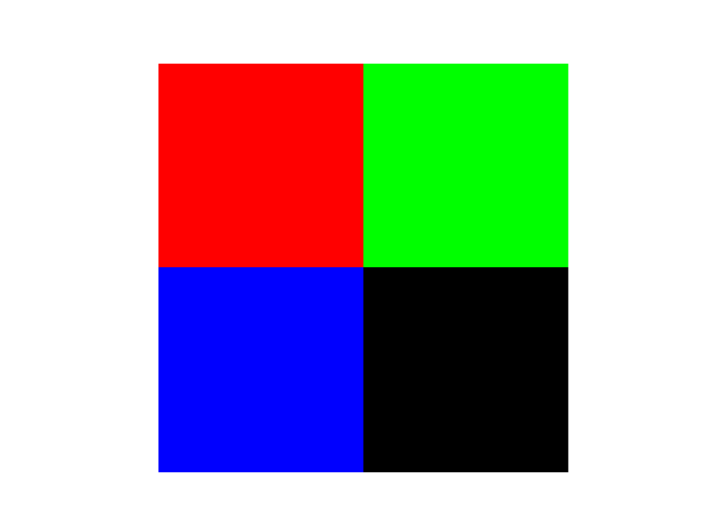
Applying the grayscale conversion formula to each pixel, we derive a new array depicting the grayscale version of the original image. This array, when visualized, illustrates the efficacy of grayscale conversion in simplifying the image data while retaining critical visual cues.
For pixel (0, 0):
Y(0, 0) = 0.2989 * 255 + 0.5870 * 0 + 0.1140 * 0 = 76.2285
Rounded to the nearest integer: 76
For pixel (0, 1):
Y(0, 1) = 0.2989 * 0 + 0.5870 * 255 + 0.1140 * 0 = 149.685
Rounded to the nearest integer: 150
For pixel (1, 0):
Y(1, 0) = 0.2989 * 0 + 0.5870 * 0 + 0.1140 * 255 = 29.07
Rounded to the nearest integer: 29
For pixel (1, 1):
Y(1, 1) = 0.2989 * 0 + 0.5870 * 0 + 0.1140 * 0 = 0
The result is:
[[[76 ,76 ,76], [150 ,150 ,150]],
[[29, 29, 29] ,[0, 0, 0]]]

To facilitate understanding, Python code is provided for creating a sample image, applying grayscale conversion, and displaying both the original and converted images.
import numpy as np
import matplotlib.pyplot as plt
import imageio
import cv2

def grayscale():
    image_array = np.array([
        [[76, 76, 76], [150, 150, 150]],
        [[29, 29, 29], [0, 0, 0]]
    ], dtype=np.uint8)
    imageio.imwrite('grayscale_image.png', image_array)
    # Display the grayscale image
    plt.imshow(image_array)
    plt.axis('off')  # Turn off axis numbers and ticks
    plt.show()

def create_image():
    # Create an array representing the image
    # Shape: Height x Width x Channels, dtype: unsigned 8-bit integer
    image_array = np.array([
        [[255, 0, 0], [0, 255, 0]],  # First row: red, green
        [[0, 0, 255], [0, 0, 0]]  # Second row: blue, black
    ], dtype=np.uint8)

    imageio.imwrite('Figure_1.png', image_array)
    # Plotting the image
    plt.imshow(image_array)
    plt.axis('off')  # Turn off axis numbers and ticks
    plt.show()

create_image()
grayscale()
In the next articles, we’ll explore more functions critical to computer vision.
Let’s us chat on X @jessicanono1